Matchups of in situ data with satellite data#
Tutorial Leads: Anna Windle (NASA, SSAI), James Allen (NASA, MSU)
Summary#
In this example we will conduct matchups of in situ AERONET-OC Rrs data with PACE OCI Rrs data. The Aerosol Robotic Network (AERONET) was developed to sustain atmospheric studies at various scales with measurements from worldwide distributed autonomous sun-photometers. This has been extended to support marine applications, called AERONET – Ocean Color (AERONET-OC), and provides the additional capability of measuring the radiance emerging from the sea (i.e., water-leaving radiance) with modified sun-photometers installed on offshore platforms like lighthouses, oceanographic and oil towers. AERONET-OC is instrumental in satellite ocean color validation activities.
In this tutorial, we will be collecting Rrs data from the Casablanca Platform AERONET-OC site located at 40.7N, 1.4W in the western Mediterranean Sea which is typically characterized as oligotrophic/mesotrophic (ocean color signals tend to strongly covary with chlorophyll a).
We will be collecting PACE OCI Rrs data in a 5x5 pixel window around the AERONET-OC site to compare to the AERONET-OC Rrs data.
Learning Objectives#
At the end of this notebook you will know:
How to access Rrs data from a specific AERONET-OC site and time
How to access PACE OCI Rrs data from a specific location and time
How to match in situ and satellite data
How to apply statistics and plot matchup data
Contents#
1. Setup#
We begin by loading a set of utility functions that work behind the scenes to do the majority of the work for us. Collapse this for now and just run the cell, but feel free to dig into it and see how things work!
Note that the get_f0 function requires the thuillier2003_f0.nc file. For the Hackweek, this is being pulled from the shared-public directory. For others trying to run the notebook, the .nc file can be found here.
Show code cell content
"""
Helper functions for PACE Hackweek Validation Tutorial.
Authors:
James Allen and Anna Windle
"""
import datetime
from pathlib import Path
import re
import earthaccess
import matplotlib.colors as mcolors
import matplotlib.pyplot as plt
import matplotlib.style as style
from matplotlib.ticker import FuncFormatter
import numpy as np
import pandas as pd
import pvlib.solarposition as sunpos
from scipy import stats, odr
import seaborn as sns
import xarray as xr
# AERONET-OC Download Constants
# Valid AERONET-OC site list
AERONET_SITES = [
'AAOT', 'Abu_Al_Bukhoosh', 'ARIAKE_TOWER', 'Bahia_Blanca', 'Banana_River',
'Blyth_NOAH', 'Casablanca_Platform', 'Chesapeake_Bay', 'COVE_SEAPRISM',
'Galata_Platform', 'Gloria', 'GOT_Seaprism', 'Grizzly_Bay',
'Gustav_Dalen_Tower', 'Helsinki_Lighthouse', 'Ieodo_Station',
'Irbe_Lighthouse', 'Kemigawa_Offshore', 'Lake_Erie', 'Lake_Okeechobee',
'Lake_Okeechobee_N', 'LISCO', 'Lucinda', 'MVCO', 'Palgrunden',
'PLOCAN_Tower', 'RdP-EsNM', 'Sacramento_River', 'San_Marco_Platform',
'Section-7_Platform', 'Socheongcho', 'South_Greenbay', 'Thornton_C-power',
'USC_SEAPRISM', 'Venise', 'WaveCIS_Site_CSI_6', 'Zeebrugge-MOW1'
]
# Get subset of AERONET columns to make it a bit more manageable (also rename)
AOC_KEEP_COLS = ["AERONET_Site", "aoc_datetime", "Site_Latitude(Degrees)",
"Site_Longitude(Degrees)", "Solar_Zenith_Angle[400nm]"]
COLUMN_RENAME = {
"Site_Latitude(Degrees)": "aoc_latitude",
"Site_Longitude(Degrees)": "aoc_longitude",
"AERONET_Site": "aoc_site",
"Solar_Zenith_Angle[400nm]": "aoc_solar_zenith"
}
# Bland-Altman/Scatterplot Constants
# Plot colors, font sizes
COLOR_PALETTE = sns.color_palette("colorblind")
COLOR_SCATTER = COLOR_PALETTE[0]
COLOR_LINE = "black" # Was "black"
COLOR_LOA = COLOR_PALETTE[2] # Was "green"
COLOR_FITLINE = COLOR_PALETTE[1] # Was "magenta"
SIZE_TITLE = 24
SIZE_AXLABEL = 20
SIZE_TEXTLABEL = 14
SHOW_LEGEND = False
# Update some defaults
plt.rcParams.update({"figure.dpi": 300})
sns.set_style("ticks", rc={"figure.dpi": 300})
sns.set_context("notebook", font_scale=1.45)
# Satellite Matchup Constants
# Short names for earthaccess lookup
SAT_LOOKUP = {
"PACE": "PACE_OCI_L2_AOP_NRT",
"AQUA": "MODISA_L2_OC",
"TERRA": "MODIST_L2_OC",
"NOAA-20": "VIIRSJ1_L2_OC",
"NOAA-21": "VIIRSJ2_L2_OC",
"SUOMI-NPP": "VIIRSN_L2_OC"
}
# List l2 flags, then build them into a dict
l2_flags_list = [
"ATMFAIL", "LAND", "PRODWARN", "HIGLINT", "HILT", "HISATZEN", "COASTZ",
"SPARE", "STRAYLIGHT", "CLDICE", "COCCOLITH", "TURBIDW", "HISOLZEN",
"SPARE", "LOWLW", "CHLFAIL", "NAVWARN", "ABSAER", "SPARE", "MAXAERITER",
"MODGLINT", "CHLWARN", "ATMWARN", "SPARE", "SEAICE", "NAVFAIL", "FILTER",
"SPARE", "BOWTIEDEL", "HIPOL", "PRODFAIL", "SPARE"]
L2_FLAGS = {flag: 1 << idx for idx, flag in enumerate(l2_flags_list)}
# Bailey and Werdell 2006 exclusion criteria
EXCLUSION_FLAGS = ["LAND", "HIGLINT", "HILT", "STRAYLIGHT", "CLDICE",
"ATMFAIL", "LOWLW", "FILTER", "NAVFAIL", "NAVWARN"]
# --------------------------------------------------------------------------- #
# General Utilities #
# --------------------------------------------------------------------------- #
def get_f0(wavelengths=None, obs_time=None, window_size=10, f0_file=None):
"""
Load the Thuillier2003 netCDF file and return F0.
Defaults to returning the full table. Input obs_time to correct for the
Earth-Sun distance.
Parameters
----------
wavelengths : array-like, optional
Wavelengths at which to compute the average irradiance.
If None, returns the full wavelength and irradiance table.
obs_time : datetime.datetime or pd.Series, optional
Observation time(s) used to correct for the Earth-Sun distance.
If None, return the mean F0 values.
window_size : int, optional
Bandpass filter size for mean filtering to selected wavelengths, in nm.
f0_file : str or pathlib.Path
Path to the f0 netCDF file of the lookup table.
Returns
-------
tuple of np.ndarray
A tuple containing:
- f0_spectra : np.ndarray
The solar irradiance values.
- f0_wave : np.ndarray
The corresponding wavelengths.
"""
if f0_file is None:
f0_file = Path("/home/jovyan/shared/pace-hackweek-2024/thuillier2003_f0.nc")
f0_file = Path(f0_file)
if not f0_file.is_file():
raise FileNotFoundError(f"File not found: {f0_file}")
ds_f0 = xr.load_dataset(f0_file)
wl = ds_f0["wavelength"].values
f0 = ds_f0["irradiance"].values
if wavelengths is not None:
f0_wave = np.array(wavelengths)
f0_spectra = bandpass_avg(f0, wl, window_size, f0_wave)
else:
f0_wave = wl
f0_spectra = f0
if obs_time is not None:
# Calculate Earth-Sun distance
es_distance = sunpos.nrel_earthsun_distance(obs_time).to_numpy()
# Deal with multiple input times
if len(pd.Series(obs_time)) > 1:
f0_spectra = f0_spectra[None, :] / es_distance[:, None]**2
else:
f0_spectra /= es_distance**2
return f0_spectra, f0_wave
def bandpass_avg(data, input_wavelengths, window_size=10,
target_wavelengths=None):
"""
Apply a band-pass filter to the data.
Parameters
----------
data : np.ndarray
1D or 2D array containing the spectral data (samples x wavelengths).
If 1D, it's assumed to be a single sample.
input_wavelengths : np.ndarray
1D array of wavelength values corresponding to the columns of data.
window_size : int, optional
Size of the window to use for averaging. Default is 10 nm.
target_wavelengths : np.ndarray, optional
1D array of target wavelengths for filtered values.
If None, the input wavelengths are used.
Returns
-------
np.ndarray
1D or 2D array containing the band-pass filtered data.
"""
data = np.atleast_2d(data)
half_window = window_size / 2
num_samples, num_input_wavelengths = data.shape
if target_wavelengths is None:
target_wavelengths = input_wavelengths
filtered_data = np.empty((num_samples, len(target_wavelengths)))
for idx, target_wl in enumerate(target_wavelengths):
start = target_wl - half_window
end = target_wl + half_window
cols_in_range = np.where((input_wavelengths >= start)
& (input_wavelengths <= end))[0]
filtered_data[:, idx] = np.nanmean(data[:, cols_in_range], axis=1)
return filtered_data if num_samples > 1 else filtered_data.flatten()
def get_column_prods(df, type_prefix):
"""Process a dataframe to create a dictionary of data products.
Parameters
----------
df : pandas DataFrame
Extracted dataframes from read_extract_file
type_prefix : str
Prefix to identify the product columns, e.g. "aoc"
Returns
-------
data_dict
dictionary mapping data product with their wavelengths and columns.
"""
data_dict = {}
pattern = rf'{type_prefix}_(\w+?)(\d*\.?\d+)?$'
for col in df.columns:
match = re.match(pattern, col)
if match:
product = match.group(1)
wavelength = match.group(2) if match.group(2) else None
if product not in data_dict:
data_dict[product] = {'wavelengths': [], 'columns': []}
data_dict[product]['columns'].append(col)
if wavelength:
if '.' in wavelength:
data_dict[product]['wavelengths'].append(float(wavelength))
else:
data_dict[product]['wavelengths'].append(int(wavelength))
return data_dict
# --------------------------------------------------------------------------- #
# AERONET_OC Utilities #
# --------------------------------------------------------------------------- #
def construct_url(aoc_site, data_level, start_date, end_date):
"""
Craft the AERONET-OC data URL.
Parameters
----------
aoc_site : str, optional
Specific AERONET-OC site (else AAOT by default)
start_date : datetime object, optional
Beginning of Aeronet data to run. Defaults to 1 Mar 2024.
end_date : datetime object, optional
End of Aeronet data to run. Defaults to today.
data_level : int, {10, 15, 20}
data quality; 20 (default, highest quality), 15, or 10.
Returns
-------
str
url to API pull
"""
# Validate inputs
if aoc_site not in AERONET_SITES:
raise ValueError(f"{aoc_site} is not an AERONET site. Available "
f"sites are: {', '.join(AERONET_SITES)}")
url = ("https://aeronet.gsfc.nasa.gov/cgi-bin/print_web_data_v3?"
f"AVG=10&LWN{data_level}=1&year={start_date.year}"
f"&month={start_date.month}&day={start_date.day}"
f"&if_no_html=1&year2={end_date.year}&month2={end_date.month}"
f"&day2={end_date.day}&site={aoc_site}")
return url
def get_data_dict(df, search_str=None):
"""Process a dataframe to create a dict and ndarray of products and waves.
Parameters
----------
df : pandas DataFrame
Extracted dataframes from read_extract_file
Returns
-------
wavelengths
numpy array of wavelengths of the data
column_map
dict of the dataframe columns associated with each wavelength
"""
if search_str is None:
search_str = "Lwn_IOP"
wavelengths = []
column_map = {}
pattern = re.compile(rf'{search_str}\[(\d+)nm\]')
for col in df.columns:
match = pattern.search(col)
if match:
wavelength = int(match.group(1))
wavelengths.append(wavelength)
column_map[wavelength] = col
return np.array(wavelengths), column_map
def process_aeronet(aoc_site="AAOT", start_date="2024-03-01", end_date=None,
data_level=15):
"""
Download and process AERONET-OC data for matchups.
Parameters
----------
aoc_site : str, optional
Specific AERONET-OC site (else AAOT by default)
start_date : datetime or str, optional
Beginning of Aeronet data to run. Defaults to "2024-03-01"
end_date : datetime or str, optional
End of Aeronet data to run. Defaults to today.
data_level : int, {10, 15, 20}
data quality; 20 (highest, but fewest), 15 (autochecked), or 10.
Returns
-------
pandas DataFrame object
Dataframe of downloaded AERONET-OC data
"""
# Set up processing
if end_date is None:
end_date = datetime.now()
start_date = pd.to_datetime(start_date, errors='raise')
end_date = pd.to_datetime(end_date, errors='raise')
# Make url
url_aoc = construct_url(aoc_site, data_level, start_date, end_date)
# Download data (skip the 5 header rows)
try:
df_aoc_full = pd.read_csv(url_aoc, delimiter=",", na_values=-999,
skiprows=5)
except Exception as e:
raise Exception(f"Could not download data. Try another station, reduce"
f" the data_level, or expand the times. (Error: {e})")
# Drop empty columns
df_aoc_full.dropna(axis=1, how='all', inplace=True)
# Parse datetimes
df_aoc_full['aoc_datetime'] = pd.to_datetime(
df_aoc_full["Date(dd-mm-yyyy)"] + ' ' + df_aoc_full["Time(hh:mm:ss)"],
format="%d:%m:%Y %H:%M:%S"
).dt.tz_localize("UTC")
# Get subset of Lwn_f/Q columns (ignore the count columns)
# Alternatively, could pull Lwn_IOP for L11 BRDF
subset_lwn = [col for col in df_aoc_full.columns
if "Lwn_f/Q" in col and "N[Lwn_f/Q" not in col]
lwn_iop = df_aoc_full[subset_lwn].values
# Now get array of wavelengths from columns
wavelengths, _ = get_data_dict(df_aoc_full[subset_lwn], "Lwn_f/Q")
# Lwn need to be normalized by F0, the mean solar irradiance at top of atm
# Note: Lwn_IOP already accounts for the Earth-Sun Distance, BRDF, and
# atmosphere transmittance
f0_spectra, _ = get_f0(wavelengths)
# Normalize to get Rrs
rrs = lwn_iop / f0_spectra[None, :]
# Generate new column names and make the rrs dataframe
aoc_rrs_cols = [f"aoc_rrs{wavelength}" for wavelength in wavelengths]
df_rrs = pd.DataFrame(rrs, columns=aoc_rrs_cols)
# Now combine with the subset of the full dataframe
df_aoc = pd.concat([df_aoc_full[AOC_KEEP_COLS], df_rrs], axis=1)
# Do some final cleanup
df_aoc.rename(columns=COLUMN_RENAME, inplace=True)
return df_aoc
# --------------------------------------------------------------------------- #
# Satellite Utilities #
# --------------------------------------------------------------------------- #
def parse_quality_flags(flag_value):
"""
Parse bitwise flag into a list of flag names.
Parameters
----------
flag_value : int
The integer representing the combined bitwise quality flags.
Returns
-------
list of str
List of flag names that are set in the flag_value.
"""
return [flag_name for flag_name, value in L2_FLAGS.items()
if (flag_value & value) != 0]
def get_fivebyfive(file, latitude, longitude, rrs_wavelengths):
"""
Get stats on a 5x5 box around station coordinates of a satellite granule.
Parameters
----------
file : earthaccess granule object
Satellite granule from earthaccess.
latitude : float
In decimal degrees for Aeronet-OC site for matchups
longitude : float
In decimal degrees (negative West) for Aeronet-OC site for matchups
rrs_wavelengths ; numpy array
Rrs wavelengths (from wavelength_3d for OCI)
Returns
-------
None.
"""
with xr.open_dataset(file, group="navigation_data") as ds_nav:
sat_lat = ds_nav['latitude'].values
sat_lon = ds_nav['longitude'].values
# Calculate the Euclidean distance for 2D lat/lon arrays
distances = np.sqrt((sat_lat - latitude)**2 + (sat_lon - longitude)**2)
# Find the index of the minimum distance
# Dimensions are (lines, pixels)
min_dist_idx = np.unravel_index(np.argmin(distances), distances.shape)
center_line, center_pixel = min_dist_idx
# Get indices for a 5x5 box around the center pixel
line_start = max(center_line - 2, 0)
line_end = min(center_line + 2 + 1, sat_lat.shape[0])
pixel_start = max(center_pixel - 2, 0)
pixel_end = min(center_pixel + 2 + 1, sat_lat.shape[1])
# Extract the data
with xr.open_dataset(file, group="geophysical_data") as ds_data:
rrs_data = ds_data['Rrs'].isel(
number_of_lines=slice(line_start, line_end),
pixels_per_line=slice(pixel_start, pixel_end)
).values
flags_data = ds_data['l2_flags'].isel(
number_of_lines=slice(line_start, line_end),
pixels_per_line=slice(pixel_start, pixel_end)
).values
# Calculate the bitwise OR of all flags in EXCLUSION_FLAGS to get a mask
exclude_mask = sum(L2_FLAGS[flag] for flag in EXCLUSION_FLAGS)
# Create a boolean mask
# True means the flag value does not contain any of the EXCLUSION_FLAGS
valid_mask = np.bitwise_and(flags_data, exclude_mask) == 0
# Get stats and averages
if valid_mask.any():
rrs_valid = rrs_data[valid_mask]
rrs_std_initial = np.std(rrs_valid, axis=0)
rrs_mean_initial = np.mean(rrs_valid, axis=0)
# Exclude spectra > 1.5 stdevs away
std_mask = np.all(
np.abs(rrs_valid - rrs_mean_initial) <= 1.5 * rrs_std_initial,
axis=1)
rrs_std = np.std(rrs_valid[std_mask], axis=0)
rrs_mean = np.mean(rrs_valid[std_mask], axis=0).flatten()
# Matchup criteria uses cv as median of 405-570nm
rrs_cv = rrs_std / rrs_mean
rrs_cv_median = np.median(rrs_cv[(rrs_wavelengths >= 405)
& (rrs_wavelengths <= 570)])
else:
rrs_cv_median = np.nan
rrs_mean = np.nan * np.empty_like(rrs_wavelengths)
# Put in dictionary of the row
row = {
"oci_datetime": pd.to_datetime(file.granule["umm"]["TemporalExtent"]
["RangeDateTime"]["BeginningDateTime"]),
"oci_cv": rrs_cv_median,
"oci_latitude": sat_lat[center_line, center_pixel],
"oci_longitude": sat_lon[center_line, center_pixel],
"oci_pixel_valid": np.sum(valid_mask)
}
# Add mean spectra to the row dictionary
for wavelength, mean_value in zip(rrs_wavelengths, rrs_mean):
key = f'oci_rrs{int(wavelength)}'
row[key] = mean_value
return row
def process_satellite(start_date, end_date, latitude, longitude, sat="PACE",
selected_dates=None):
"""
Download and process satellite data for matchups.
Caution: If the date or coordinates aren't formatted correctly, it might
pull a huge granule list and take forever to run. If it takes more than 45
seconds to print the number of granules, just kill the process.
Uses the earthaccess package. Defaults to the PACE OCI L2 IOP datasets,
but other satellites can be used if they have a corresponding short_name
in the SAT_LOOKUP dictionary.
Workflow:
1. Get list of matchup granules
2. Loop through each file and:
2a. Find closest pixel to station, extract 5x5 pixel box
2b. Exclude pixels based on l2_flags
2c. Filtered mean to get single spectra
2d. Compute statistics and save data row
3. Organize output pandas dataframe
Parameters
----------
start_date : datetime or str
Beginning of Aeronet data to run.
end_date : datetime or str, optional
End of Aeronet data to run.
latitude : float
In decimal degrees for Aeronet-OC site for matchups
longitude : float
In decimal degrees (negative West) for Aeronet-OC site for matchups
sat : str
Name of satellite to search. Must be in SAT_LOOKUP dict constant.
selected_dates : list of str, optional
If given, only pull granules if the dates are in this list
Returns
-------
pandas DataFrame object
Flattened table of all satellite granule matchups.
"""
# Look up short name from constants
if sat not in SAT_LOOKUP.keys():
raise ValueError(f"{sat} is not in the lookup dictionary. Available "
f"sats are: {', '.join(SAT_LOOKUP)}")
short_name = SAT_LOOKUP[sat]
# Format search parameters
time_bounds = (f"{start_date}T00:00:00", f"{end_date}T23:59:59")
# Run Earthaccess data search
results = earthaccess.search_data(point=(longitude, latitude),
temporal=time_bounds,
short_name=short_name)
if selected_dates is not None:
filtered_results = [
result for result in results
if result["umm"]["TemporalExtent"]["RangeDateTime"]["BeginningDateTime"][:10]
in selected_dates
]
print(f"Filtered to {len(filtered_results)} Granules.")
files = earthaccess.open(filtered_results)
else:
files = earthaccess.open(results)
# Pull out Rrs wavelengths for easier processing
with xr.open_dataset(files[0], group="sensor_band_parameters") as ds_bands:
rrs_wavelengths = ds_bands["wavelength_3d"].values
# Loop through files and process
sat_rows = []
for idx, file in enumerate(files):
granule_date = pd.to_datetime(file.granule["umm"]["TemporalExtent"]
["RangeDateTime"]["BeginningDateTime"])
print(f"Running Granule: {granule_date}")
row = get_fivebyfive(file, latitude, longitude, rrs_wavelengths)
sat_rows.append(row)
return pd.DataFrame(sat_rows)
# --------------------------------------------------------------------------- #
# Matchup Utilities #
# --------------------------------------------------------------------------- #
def match_data(df_sat, df_aoc, cv_max=0.15, senz_max=60.0,
min_percent_valid=55.0, max_time_diff=180, std_max=1.5):
"""Create matchup dataframe based on selection criteria.
Parameters
----------
df_sat : pandas dataframe
Satellite data from flat validation file.
df_aoc : pandas dataframe
Field data from flat validation file.
cv_max : float, default 0.15
Maximum coefficient of variation (stdev/mean) for sat data.
senz_max : float, default 60.0
Maximum sensor zenith for sat data.
min_percent_valid : float, default 55.0
Minimum percentage of valid satellite pixels.
max_time_diff : int, default 180
Maximum time difference (minutes) between sat and field matchup.
std_max : float, default 1.5
If multiple valid field matchups, select within std_max stdevs of mean.
Returns
-------
pandas dataframe of matchups for product
"""
# Setup
time_window = pd.Timedelta(minutes=max_time_diff)
df_match_list = []
# Filter Field data based on Solar Zenith
df_aoc_filtered = df_aoc[df_aoc['aoc_solar_zenith'] <= senz_max]
# Filter satellite data based on cv threshold
df_sat_filtered = df_sat[df_sat['oci_cv'] <= cv_max]
# Filter satellite data based on percent good pixels
df_sat_filtered = df_sat_filtered[
df_sat_filtered['oci_pixel_valid'] >= min_percent_valid * 25 / 100]
for _, sat_row in df_sat_filtered.iterrows():
# Filter field data based on time difference and coordinates
time_diff = abs(df_aoc_filtered['aoc_datetime']-sat_row['oci_datetime'])
within_time = time_diff <= time_window
within_lat = 0.2 >= abs(
df_aoc_filtered['aoc_latitude'] - sat_row['oci_latitude'])
within_lon = 0.2 >= abs(
df_aoc_filtered['aoc_longitude'] - sat_row['oci_longitude'])
field_matches = df_aoc_filtered[within_time & within_lat & within_lon]
if field_matches.shape[0] > 5:
# Filter by Standard Deviation for rrs columns
rrs_cols = [col for col in field_matches.columns
if col.startswith('aoc_rrs')]
if rrs_cols:
mean_spectra = field_matches[rrs_cols].mean(axis=0)
std_spectra = field_matches[rrs_cols].std(axis=0)
within_std = (abs(field_matches[rrs_cols] - mean_spectra)
<= std_max * std_spectra)
field_matches = field_matches[within_std.all(axis=1)]
if not field_matches.empty:
# Select the best match based on time delta
time_diff = abs(
field_matches['aoc_datetime']-sat_row['oci_datetime'])
best_match = field_matches.loc[time_diff.idxmin()]
df_match_list.append({**best_match.to_dict(), **sat_row.to_dict()})
df_match = pd.DataFrame(df_match_list)
return df_match
# --------------------------------------------------------------------------- #
# Plotting Utilities #
# --------------------------------------------------------------------------- #
def compute_bland_altman_metrics(xx, yy, xx_unc_modl, yy_unc_modl):
"""
Compute metrics for Bland-Altman plot.
Parameters
----------
xx : array
Array of X data values.
yy : array
Array of Y data values.
xx_unc_modl : float
Uncertainty in X.
yy_unc_modl : float
Uncertainty in Y.
Returns
-------
dict
Dictionary of Bland-Altman metrics.
"""
jj = (xx + yy) / 2
kk = (yy - xx) / np.sqrt((xx_unc_modl**2) + (yy_unc_modl**2))
meanbias = np.mean(kk)
stdbias = np.std(kk)
LOAlow = meanbias - stdbias
LOAhgh = meanbias + stdbias
ba_stat, ba_p = stats.spearmanr(jj, kk)
ba_independ = ba_p > 0.05
return {
"count": kk.shape[0],
"jj": jj,
"kk": kk,
"meanbias": meanbias,
"LOAlow": LOAlow,
"LOAhgh": LOAhgh,
"ba_stat": ba_stat,
"ba_p": ba_p,
"ba_independ": ba_independ
}
def compute_regression_metrics(xx, yy, is_type2=False):
"""
Compute regression metrics using specified type.
Parameters
----------
xx : array
Array of X data values.
yy : array
Array of Y data values.
is_type2 : bool, optional
Whether to use Type 2 regression (orthogonal distance regression).
Default is False, for Type 1 regression (ordinary least squares).
Returns
-------
dict
Dictionary of regression metrics.
"""
if is_type2:
# Perform Type 2 regression (orthogonal distance regression)
def linear_model(B, x):
"""
Linear function y = m*x + b.
B is a vector of the parameters.
x is an array of the current x values.
x is in the same format as the x passed to Data or RealData.
Return an array in the same format as y passed to Data or RealData.
"""
return B[0] * x + B[1]
# Create a model instance
linear = odr.Model(linear_model)
# Create a RealData object using the data
data = odr.RealData(xx, yy)
# Set up ODR with the model and data
odr_instance = odr.ODR(data, linear, beta0=[1., 0.])
# Run the regression
odr_result = odr_instance.run()
slope = odr_result.beta[0]
intercept = odr_result.beta[1]
else:
# Perform Type 1 regression (ordinary least squares)
regress_result = stats.linregress(xx, yy)
slope = regress_result.slope
intercept = regress_result.intercept
spearman_r = stats.spearmanr(xx, yy)
pearson_r = stats.pearsonr(xx, yy)
rmse_all = np.sqrt(np.mean((yy - xx) ** 2))
mae_all = np.mean(np.abs(yy - xx))
return {
"count": len(xx),
"slope": slope,
"intercept": intercept,
"r_spear": spearman_r.correlation,
"r_pear": pearson_r[0],
"rmse": rmse_all,
"mae": mae_all
}
def add_text_annotations(ax, text_lines, position='top right',
fontsize=SIZE_TEXTLABEL):
"""
Add text annotations to the plot.
Parameters
----------
ax : Axes
The axis to add text to.
text_lines : list of str
List of strings to be displayed as text.
position : str, default 'top right'
Position of the text on the plot.
fontsize : int, default 12
Font size of the text.
"""
if position == 'top right':
x = 0.95
y = 0.95
ha = 'right'
va = 'top'
elif position == 'top left':
x = 0.05
y = 0.95
ha = 'left'
va = 'top'
elif position == 'bottom left':
x = 0.05
y = 0.05
ha = 'left'
va = 'bottom'
elif position == 'bottom right':
x = 0.95
y = 0.05
ha = 'right'
va = 'bottom'
text = '\n'.join(text_lines)
ax.text(
x, y, text, transform=ax.transAxes, fontsize=fontsize,
verticalalignment=va, horizontalalignment=ha,
bbox=dict(facecolor='white', alpha=0.6, edgecolor='none')
)
def setup_plot(label):
"""
Set up the plot with titles and labels.
Parameters
----------
label : str
Title of the plot.
Returns
-------
tuple
Figure and axes of the plot.
"""
style.use('seaborn-v0_8-whitegrid')
fig, (ax1, ax2) = plt.subplots(1, 2, figsize=(16, 6), layout="constrained")
fig.suptitle(label, fontsize=22)
return fig, ax1, ax2
def format_ticks(ax):
"""Format the tick labels on the axes to be more readable."""
ax.xaxis.set_major_formatter(FuncFormatter(lambda x, _: f'{x:.3g}'))
ax.yaxis.set_major_formatter(FuncFormatter(lambda y, _: f'{y:.3g}'))
ax.tick_params(axis='both', which='major', width=2, length=6)
ax.spines['top'].set_linewidth(2)
ax.spines['right'].set_linewidth(2)
ax.spines['left'].set_linewidth(2)
ax.spines['bottom'].set_linewidth(2)
def plot_bland_altman(ax1, metrics, binscale, scat, xx_unc_modl,
x_label="x", y_label="y"):
"""
Plot Bland-Altman plot.
Parameters
----------
ax1 : Axes
Axis for the Bland-Altman plot.
metrics : dict
Bland-Altman metrics.
binscale : float
Scaling factor for bin size.
scat : bool
If False, plot as 2D histogram.
xx_unc_modl : float
Uncertainty in X.
x_label : string, default "x"
String for labels for x data
y_label : string, default "y"
String for labels for y data
"""
jj = metrics["jj"]
kk = metrics["kk"]
npoints = metrics["count"]
meanbias = metrics["meanbias"]
LOAlow = metrics["LOAlow"]
LOAhgh = metrics["LOAhgh"]
ba_independ = metrics["ba_independ"]
ba_stat = metrics["ba_stat"]
nbin = int(0.5 * binscale * np.sqrt(len(jj)))
min_kk = meanbias - 5 * np.std(kk)
max_kk = meanbias + 5 * np.std(kk)
gamma = 0.5
if scat:
min_jj = np.min(jj)
max_jj = np.max(jj)
lineclr, loaclr, fitclr = (COLOR_LINE, COLOR_LOA, COLOR_FITLINE)
ax1.scatter(jj, kk, color=COLOR_SCATTER)
ax1.set_xlim([min_jj, max_jj])
ax1.set_ylim([min_kk, max_kk])
else:
jj_sorted = np.sort(jj)
min_jj = jj_sorted[int(0.01 * len(jj))]
max_jj = jj_sorted[int(0.99 * len(jj))]
lineclr, loaclr, fitclr = ('white', 'yellow', 'cyan')
h = ax1.hist2d(jj, kk, bins=(nbin, nbin),
norm=mcolors.PowerNorm(gamma), cmap=plt.cm.inferno,
range=[[min_jj, max_jj], [min_kk, max_kk]])
plt.colorbar(h[3], ax=ax1)
ax1.set_title('Bland-Altman plot', fontsize=SIZE_TITLE)
ylabel = ('Uncertainty normalized bias' if xx_unc_modl != np.sqrt(0.5)
else f'Bias, ${y_label}-{x_label}$')
ax1.set_ylabel(ylabel, fontsize=SIZE_AXLABEL)
ax1.set_xlabel(f'Paired mean, $({x_label}+{y_label})/2$',
fontsize=SIZE_AXLABEL)
ax1.plot([min_jj, max_jj], [0, 0],
color=lineclr, linestyle='solid', linewidth=4.0)
if ba_independ:
ax1.plot([min_jj, max_jj], [meanbias, meanbias],
color=fitclr, linestyle='dashed', linewidth=3.0,
label='Mean Bias')
ax1.plot([min_jj, max_jj], [LOAlow, LOAlow],
color=loaclr, linestyle='dashed', linewidth=2.0,
label='Lower LOA')
ax1.plot([min_jj, max_jj], [LOAhgh, LOAhgh],
color=loaclr, linestyle='dashed', linewidth=2.0,
label='Upper LOA')
ax1.fill_between([min_jj, max_jj], LOAlow, LOAhgh,
color=loaclr, alpha=0.1)
else:
ba_regress_result = stats.linregress(jj, kk)
ba_min_fit_yy = (ba_regress_result.slope * min_jj
+ ba_regress_result.intercept)
ba_max_fit_yy = (ba_regress_result.slope * max_jj
+ ba_regress_result.intercept)
ax1.plot([min_jj, max_jj], [ba_min_fit_yy, ba_max_fit_yy],
color=fitclr, linestyle='dashed', linewidth=3.0,
label='Linear Fit')
if SHOW_LEGEND:
ax1.legend()
ax1.grid(True)
format_ticks(ax1)
text_lines = [
f"Number of Points: {npoints}",
f"Mean Bias: {meanbias:.2e}",
f"Limits of Agreement: [{LOAlow:.2e}, {LOAhgh:.2e}]",
f"Rank Correlation: {ba_stat:.3f}",
"Bias Independent" if ba_independ else "Bias Dependent"
]
add_text_annotations(ax1, text_lines, position='bottom right')
def plot_scatter(ax2, xx, yy, regress_metrics, binscale, scat,
x_label="x", y_label="y"):
"""
Plot scatter plot with regression line.
Parameters
----------
ax2 : Axes
Axis for the scatter plot.
xx : array
Array of X data values.
yy : array
Array of Y data values.
regress_metrics : dict
Regression metrics.
binscale : float
Scaling factor for bin size.
scat : bool
If False, plot as 2D histogram.
x_label : string, default "x"
String for labels for x data
y_label : string, default "y"
String for labels for y data
"""
nbin = int(0.5 * binscale * np.sqrt(len(xx)))
min_val = min(np.min(xx), np.min(yy))
max_val = max(np.max(xx), np.max(yy))
gamma = 0.5
if scat:
ax2.scatter(xx, yy, color=COLOR_SCATTER)
ax2.set_xlim([min_val, max_val])
ax2.set_ylim([min_val, max_val])
else:
g = ax2.hist2d(xx, yy, bins=(nbin, nbin),
norm=mcolors.PowerNorm(gamma), cmap=plt.cm.inferno,
range=[[min_val, max_val], [min_val, max_val]])
plt.colorbar(g[3], ax=ax2)
ax2.set_title('Scatterplot', fontsize=SIZE_TITLE)
ax2.set_xlabel(f'${x_label}$', fontsize=SIZE_AXLABEL)
ax2.set_ylabel(f'${y_label}$', fontsize=SIZE_AXLABEL)
ax2.plot([min_val, max_val], [min_val, max_val],
color=COLOR_LINE, linestyle='solid', linewidth=4.0)
slope = regress_metrics["slope"]
intercept = regress_metrics["intercept"]
min_fit_yy = slope * min_val + intercept
max_fit_yy = slope * max_val + intercept
ax2.plot([min_val, max_val], [min_fit_yy, max_fit_yy],
color=COLOR_FITLINE, linestyle='dashed', linewidth=3.0,
label='Regression Line')
if SHOW_LEGEND:
ax2.legend()
ax2.grid(True)
format_ticks(ax2)
text_lines = [
f"Slope: {slope:.3f}",
f"Intercept: {intercept:.2e}",
f"Linear Correlation: {regress_metrics['r_pear']:.3f}",
f"Rank Correlation: {regress_metrics['r_spear']:.3f}",
f"RMSE: {regress_metrics['rmse']:.2e}",
f"MAE: {regress_metrics['mae']:.2e}"
]
add_text_annotations(ax2, text_lines, position='bottom right')
def plot_BAvsScat(x_input, y_input, label='',
saveplot=None, scat=True, binscale=1.0,
xx_unc_modl=np.sqrt(0.5), yy_unc_modl=np.sqrt(0.5),
x_label="x", y_label="y", is_type2=True):
"""
Routine to plot paired data as Bland-Altman and scatter plot.
Parameters
----------
x_input : array-like
Array of X data values.
y_input : array-like
Corresponding array of Y data values.
label : string, default ''
Text label for plotting.
saveplot : string, default None
Set to save plot in ../output/ with the string as the filename.
scat : boolean, default True
Make a 2D histogram if False, regular scatter plot if True.
binscale : float, default 1.0
Scaling factor for how many bins to include in a 2D histogram.
xx_unc_modl : float, default np.sqrt(0.5)
Uncertainty in X.
yy_unc_modl : float, default np.sqrt(0.5)
Uncertainty in Y.
x_label : string, default "x"
String for labels for x data
y_label : string, default "y"
String for labels for y data
Returns
-------
dict
Dictionary of computed statistics.
"""
xx = np.asarray(x_input)
yy = np.asarray(y_input)
valid_indices = (np.isfinite(x_input) & np.isfinite(y_input)
& (x_input != -999) & (y_input != -999))
xx = x_input[valid_indices]
yy = y_input[valid_indices]
ba_metrics = compute_bland_altman_metrics(xx, yy, xx_unc_modl, yy_unc_modl)
regress_metrics = compute_regression_metrics(xx, yy, is_type2=is_type2)
fig, ax1, ax2 = setup_plot(label)
plot_bland_altman(ax1, ba_metrics, binscale, scat, xx_unc_modl,
x_label, y_label)
plot_scatter(ax2, xx, yy, regress_metrics, binscale, scat,
x_label, y_label)
if saveplot is not None:
figpath = Path("../output") / saveplot
fig.savefig(figpath)
print('Saved figure to:', figpath)
plt.show()
return {
"Number_of_Points": ba_metrics["count"],
"Scale_Independence": ba_metrics["ba_independ"],
"Mean_Bias": ba_metrics["meanbias"],
"Limits_of_Agreement_low": (ba_metrics["LOAlow"]
if ba_metrics["ba_independ"]
else float("nan")),
"Limits_of_Agreement_high": (ba_metrics["LOAhgh"]
if ba_metrics["ba_independ"]
else float("nan")),
"Linear_Slope": regress_metrics["slope"],
"Linear_Intercept": regress_metrics["intercept"],
"Linear_Correlation": regress_metrics["r_pear"],
"Rank_Correlation": regress_metrics["r_spear"],
"RMSE": regress_metrics["rmse"],
"MAE": regress_metrics["mae"]
}
2. Process AERONET-OC data#
We will use the function process_aeronet to download and process AERONET-OC data from the ‘Casablanca_Platform’ site. We will filter Level 1.5 data from the dates June 1, 2024 to July 31, 2024. This function will output a pandas dataframe of every AERONET-OC record between the dates.
There are three “levels” of AERONET-OC data in terms of data quality: 1, 1.5, and 2. If a complete measurement sequence with the instruments is able to be performed, it is collected and stored as Level 1. These data are then passed through an automated quality control system and stored as Level 1.5 if they pass all tests. Finally, Level 2 data are data from Level 1.5 that are subsequently screened by an experienced scientist and validated. We’ll be using Level 1.5 data to pull as much good quality data as possible without the time lag for manual validation. More information on AERONET-OC levels can be found in Zibordi et al., 2009.
aoc_cb = process_aeronet(aoc_site="Casablanca_Platform",
                start_date="2024-06-01", end_date="2024-07-31",
                data_level=15)
aoc_cb.head()
| aoc_site | aoc_datetime | aoc_latitude | aoc_longitude | aoc_solar_zenith | aoc_rrs400 | aoc_rrs412 | aoc_rrs443 | aoc_rrs490 | aoc_rrs510 | aoc_rrs560 | aoc_rrs620 | aoc_rrs667 | aoc_rrs779 | aoc_rrs865 | aoc_rrs1020 | |
|---|---|---|---|---|---|---|---|---|---|---|---|---|---|---|---|---|
| 0 | Casablanca_Platform | 2024-06-02 11:02:49+00:00 | 40.717 | 1.358 | 20.961198 | 0.006671 | 0.007168 | 0.006529 | 0.005395 | 0.003582 | 0.001815 | 0.000383 | 0.000255 | 0.000073 | 0.000054 | 0.000039 |
| 1 | Casablanca_Platform | 2024-06-02 11:07:35+00:00 | 40.717 | 1.358 | 20.501438 | 0.006907 | 0.007283 | 0.006486 | 0.005382 | 0.003673 | 0.001843 | 0.000447 | 0.000317 | 0.000103 | 0.000116 | 0.000076 |
| 2 | Casablanca_Platform | 2024-06-02 12:31:52+00:00 | 40.717 | 1.358 | 20.424684 | 0.007173 | 0.007603 | 0.006800 | 0.005645 | 0.003774 | 0.001888 | 0.000490 | 0.000313 | 0.000108 | 0.000193 | 0.000104 |
| 3 | Casablanca_Platform | 2024-06-02 13:31:51+00:00 | 40.717 | 1.358 | 28.254349 | 0.007199 | 0.007584 | 0.006990 | 0.005811 | 0.003998 | 0.002078 | 0.000634 | 0.000347 | 0.000171 | 0.000242 | 0.000089 |
| 4 | Casablanca_Platform | 2024-06-02 14:02:47+00:00 | 40.717 | 1.358 | 33.420386 | 0.007052 | 0.007523 | 0.006940 | 0.005631 | 0.003993 | 0.002090 | 0.000436 | 0.000318 | 0.000130 | 0.000125 | 0.000172 |
3. Process PACE OCI data#
We will use the function process_satellite to search for PACE_OCI_L2_AOP_NRT data using earthacces within the specified time range and at the (lat,lon) coordinate of the Casablanca_Platform AERONET-OC site. This function finds the closest pixel and extracts all data within a 5x5 pixel window, excludes pixels based on L2 flags, calculates the mean to retrive a single Rrs spectra, and computes matchup statistics. The function outputs a pandas dataframe of every PACE_OCI_L2_AOP_NRT Rrs spectra for the specified time range. We’ll also include an optional list of unique date strings from the AERONET-OC dataframe to “skip” the granules that don’t have any field data associated with them.
# Pull out coordinates
aoc_lat = aoc_cb["aoc_latitude"][0]
aoc_lon = aoc_cb["aoc_longitude"][0]

# Pull out unique days
unique_days = aoc_cb["aoc_datetime"].dt.date.unique()
unique_days_str = [day.strftime('%Y-%m-%d') for day in unique_days]

sat_cb = process_satellite(start_date="2024-06-01", end_date="2024-07-31",
                  latitude=aoc_lat, longitude=aoc_lon, sat="PACE",
                  selected_dates=unique_days_str)
Filtered to 70 Granules.
Running Granule: 2024-06-02 12:32:12+00:00
Running Granule: 2024-06-03 11:33:41+00:00
Running Granule: 2024-06-03 13:07:01+00:00
Running Granule: 2024-06-04 12:03:29+00:00
Running Granule: 2024-06-05 12:38:15+00:00
Running Granule: 2024-06-10 12:15:27+00:00
Running Granule: 2024-06-13 12:21:23+00:00
Running Granule: 2024-06-14 11:17:49+00:00
Running Granule: 2024-06-14 12:56:08+00:00
Running Granule: 2024-06-15 11:52:33+00:00
Running Granule: 2024-06-16 12:27:17+00:00
Running Granule: 2024-06-17 11:23:41+00:00
Running Granule: 2024-06-17 13:01:59+00:00
Running Granule: 2024-06-18 11:58:24+00:00
Running Granule: 2024-06-20 11:29:32+00:00
Running Granule: 2024-06-20 13:07:51+00:00
Running Granule: 2024-06-21 12:04:15+00:00
Running Granule: 2024-06-23 11:35:22+00:00
Running Granule: 2024-06-23 13:13:40+00:00
Running Granule: 2024-06-24 12:10:03+00:00
Running Granule: 2024-06-25 12:44:45+00:00
Running Granule: 2024-06-26 11:41:08+00:00
Running Granule: 2024-06-26 13:19:27+00:00
Running Granule: 2024-06-27 12:15:50+00:00
Running Granule: 2024-06-28 12:50:31+00:00
Running Granule: 2024-06-29 11:46:54+00:00
Running Granule: 2024-06-29 13:25:13+00:00
Running Granule: 2024-06-30 12:21:35+00:00
Running Granule: 2024-07-01 11:17:57+00:00
Running Granule: 2024-07-01 12:56:16+00:00
Running Granule: 2024-07-02 11:52:38+00:00
Running Granule: 2024-07-03 12:27:18+00:00
Running Granule: 2024-07-04 11:23:40+00:00
Running Granule: 2024-07-04 13:01:59+00:00
Running Granule: 2024-07-05 11:58:20+00:00
Running Granule: 2024-07-06 12:33:00+00:00
Running Granule: 2024-07-07 11:29:22+00:00
Running Granule: 2024-07-07 13:07:40+00:00
Running Granule: 2024-07-08 12:03:55+00:00
Running Granule: 2024-07-09 12:38:34+00:00
Running Granule: 2024-07-10 11:34:54+00:00
Running Granule: 2024-07-10 13:13:12+00:00
Running Granule: 2024-07-11 12:09:32+00:00
Running Granule: 2024-07-12 12:44:10+00:00
Running Granule: 2024-07-13 11:40:30+00:00
Running Granule: 2024-07-13 13:18:48+00:00
Running Granule: 2024-07-14 12:15:08+00:00
Running Granule: 2024-07-15 12:49:45+00:00
Running Granule: 2024-07-16 11:46:03+00:00
Running Granule: 2024-07-16 13:24:22+00:00
Running Granule: 2024-07-17 12:20:40+00:00
Running Granule: 2024-07-18 11:17:53+00:00
Running Granule: 2024-07-18 12:56:12+00:00
Running Granule: 2024-07-19 11:51:35+00:00
Running Granule: 2024-07-20 12:26:12+00:00
Running Granule: 2024-07-21 11:22:29+00:00
Running Granule: 2024-07-21 13:00:48+00:00
Running Granule: 2024-07-22 11:57:04+00:00
Running Granule: 2024-07-23 12:31:40+00:00
Running Granule: 2024-07-24 11:32:57+00:00
Running Granule: 2024-07-24 13:06:15+00:00
Running Granule: 2024-07-25 12:02:32+00:00
Running Granule: 2024-07-26 12:37:07+00:00
Running Granule: 2024-07-27 11:38:24+00:00
Running Granule: 2024-07-27 13:11:42+00:00
Running Granule: 2024-07-28 12:07:59+00:00
Running Granule: 2024-07-29 12:42:29+00:00
Running Granule: 2024-07-30 11:43:44+00:00
Running Granule: 2024-07-30 13:17:02+00:00
Running Granule: 2024-07-31 12:13:17+00:00
/tmp/ipykernel_312/3719509098.py:465: RuntimeWarning: invalid value encountered in divide
  rrs_cv = rrs_std / rrs_mean
/srv/conda/envs/notebook/lib/python3.10/site-packages/numpy/core/_methods.py:206: RuntimeWarning: Degrees of freedom <= 0 for slice
  ret = _var(a, axis=axis, dtype=dtype, out=out, ddof=ddof,
/srv/conda/envs/notebook/lib/python3.10/site-packages/numpy/core/_methods.py:163: RuntimeWarning: invalid value encountered in divide
  arrmean = um.true_divide(arrmean, div, out=arrmean,
/srv/conda/envs/notebook/lib/python3.10/site-packages/numpy/core/_methods.py:195: RuntimeWarning: invalid value encountered in divide
  ret = um.true_divide(
/srv/conda/envs/notebook/lib/python3.10/site-packages/numpy/core/fromnumeric.py:3504: RuntimeWarning: Mean of empty slice.
  return _methods._mean(a, axis=axis, dtype=dtype,
/srv/conda/envs/notebook/lib/python3.10/site-packages/numpy/core/_methods.py:121: RuntimeWarning: invalid value encountered in divide
  ret = um.true_divide(
/tmp/ipykernel_312/3719509098.py:465: RuntimeWarning: divide by zero encountered in divide
  rrs_cv = rrs_std / rrs_mean
sat_cb.head()
| oci_datetime | oci_cv | oci_latitude | oci_longitude | oci_pixel_valid | oci_rrs339 | oci_rrs341 | oci_rrs344 | oci_rrs346 | oci_rrs348 | ... | oci_rrs706 | oci_rrs707 | oci_rrs708 | oci_rrs709 | oci_rrs711 | oci_rrs712 | oci_rrs713 | oci_rrs714 | oci_rrs717 | oci_rrs719 | |
|---|---|---|---|---|---|---|---|---|---|---|---|---|---|---|---|---|---|---|---|---|---|
| 0 | 2024-06-02 12:32:12+00:00 | 0.018682 | 40.718674 | 1.354624 | 25 | 0.003125 | 0.001464 | 0.001523 | 0.001712 | 0.002017 | ... | 0.000041 | 0.000030 | 0.000024 | 0.000018 | 0.000010 | 0.000003 | 0.000011 | 0.000038 | 0.000232 | 0.000408 |
| 1 | 2024-06-03 11:33:41+00:00 | 0.016600 | 40.717136 | 1.369991 | 25 | 0.000713 | -0.001183 | -0.000998 | -0.000949 | -0.000604 | ... | -0.000306 | -0.000306 | -0.000299 | -0.000280 | -0.000269 | -0.000268 | -0.000268 | -0.000295 | -0.000213 | -0.000056 |
| 2 | 2024-06-03 13:07:01+00:00 | 0.034840 | 40.717754 | 1.348150 | 25 | 0.000256 | -0.002797 | -0.003166 | -0.003049 | -0.002762 | ... | -0.000128 | -0.000144 | -0.000157 | -0.000158 | -0.000156 | -0.000153 | -0.000136 | -0.000094 | 0.000221 | 0.000514 |
| 3 | 2024-06-04 12:03:29+00:00 | 0.033988 | 40.713097 | 1.353367 | 11 | -0.001250 | -0.002048 | -0.001527 | -0.001212 | -0.000768 | ... | -0.000107 | -0.000112 | -0.000114 | -0.000113 | -0.000112 | -0.000112 | -0.000110 | -0.000110 | -0.000021 | 0.000106 |
| 4 | 2024-06-05 12:38:15+00:00 | 0.000000 | 40.712395 | 1.359444 | 1 | 0.001784 | 0.000006 | 0.000096 | 0.000278 | 0.000552 | ... | -0.000080 | -0.000074 | -0.000066 | -0.000060 | -0.000060 | -0.000072 | -0.000078 | -0.000082 | 0.000044 | 0.000182 |
5 rows × 189 columns
3. Apply matchup code#
We will use the function match_data to create a matchup dataframe based on selection criteria. This function defaults to using the Bailey and Werdell 2006 matchup criteria, which reduces the measurements made at a given station to one representative sample for validating against the satellite spectra. Data are filtered based on the solar zenith angle, their noise level, and the time difference (here 180 minutes from the satellite overpass). Potential satellite matchups are also reduced based on the signal to noise level of the 5x5 pixel aggregation.
?match_data
matchups = match_data(sat_cb, aoc_cb, cv_max=0.60, senz_max=60.0,
                      min_percent_valid=55.0, max_time_diff=180, std_max=1.5)
matchups
| aoc_site | aoc_datetime | aoc_latitude | aoc_longitude | aoc_solar_zenith | aoc_rrs400 | aoc_rrs412 | aoc_rrs443 | aoc_rrs490 | aoc_rrs510 | ... | oci_rrs706 | oci_rrs707 | oci_rrs708 | oci_rrs709 | oci_rrs711 | oci_rrs712 | oci_rrs713 | oci_rrs714 | oci_rrs717 | oci_rrs719 | |
|---|---|---|---|---|---|---|---|---|---|---|---|---|---|---|---|---|---|---|---|---|---|
| 0 | Casablanca_Platform | 2024-06-02 12:31:52+00:00 | 40.717 | 1.358 | 20.424684 | 0.007173 | 0.007603 | 0.006800 | 0.005645 | 0.003774 | ... | 0.000041 | 3.000062e-05 | 0.000024 | 0.000018 | 0.000010 | 0.000003 | 0.000011 | 0.000038 | 0.000232 | 0.000408 |
| 1 | Casablanca_Platform | 2024-06-03 11:32:00+00:00 | 40.717 | 1.358 | 18.711231 | 0.007375 | 0.007822 | 0.006910 | 0.005686 | 0.003827 | ... | -0.000306 | -3.056657e-04 | -0.000299 | -0.000280 | -0.000269 | -0.000268 | -0.000268 | -0.000295 | -0.000213 | -0.000056 |
| 2 | Casablanca_Platform | 2024-06-03 12:07:53+00:00 | 40.717 | 1.358 | 18.679252 | 0.007319 | 0.007779 | 0.006967 | 0.005692 | 0.003687 | ... | -0.000128 | -1.444989e-04 | -0.000157 | -0.000158 | -0.000156 | -0.000153 | -0.000136 | -0.000094 | 0.000221 | 0.000514 |
| 3 | Casablanca_Platform | 2024-06-13 12:09:40+00:00 | 40.717 | 1.358 | 17.843898 | 0.007230 | 0.007573 | 0.006626 | 0.005214 | 0.003381 | ... | 0.000006 | 9.313226e-10 | -0.000007 | -0.000003 | -0.000009 | -0.000014 | -0.000011 | -0.000016 | 0.000058 | 0.000149 |
| 4 | Casablanca_Platform | 2024-06-16 12:29:38+00:00 | 40.717 | 1.358 | 18.983302 | 0.007927 | 0.008355 | 0.007261 | 0.005747 | 0.003678 | ... | 0.000005 | -2.749264e-06 | -0.000007 | -0.000011 | -0.000014 | -0.000018 | -0.000014 | -0.000010 | 0.000093 | 0.000207 |
| 5 | Casablanca_Platform | 2024-06-18 12:30:02+00:00 | 40.717 | 1.358 | 18.939030 | 0.007971 | 0.008290 | 0.007422 | 0.005780 | 0.003872 | ... | -0.000276 | -2.729992e-04 | -0.000263 | -0.000248 | -0.000240 | -0.000237 | -0.000248 | -0.000283 | -0.000284 | -0.000172 |
| 6 | Casablanca_Platform | 2024-06-21 12:06:23+00:00 | 40.717 | 1.358 | 17.474860 | 0.007524 | 0.007917 | 0.007559 | 0.006464 | 0.004480 | ... | 0.000058 | 4.775077e-05 | 0.000037 | 0.000026 | 0.000015 | 0.000007 | 0.000016 | 0.000042 | 0.000227 | 0.000384 |
| 7 | Casablanca_Platform | 2024-06-24 13:16:19+00:00 | 40.717 | 1.358 | 24.368037 | 0.007961 | 0.008831 | 0.008300 | 0.006934 | 0.004899 | ... | 0.000006 | 1.000861e-06 | -0.000005 | -0.000009 | -0.000008 | -0.000024 | -0.000024 | -0.000019 | 0.000106 | 0.000246 |
| 8 | Casablanca_Platform | 2024-06-26 12:07:21+00:00 | 40.717 | 1.358 | 17.578107 | 0.007628 | 0.008228 | 0.007718 | 0.006388 | 0.004236 | ... | -0.000226 | -2.393325e-04 | -0.000245 | -0.000240 | -0.000235 | -0.000240 | -0.000231 | -0.000209 | 0.000102 | 0.000439 |
| 9 | Casablanca_Platform | 2024-06-26 13:31:32+00:00 | 40.717 | 1.358 | 26.676126 | 0.007576 | 0.008119 | 0.007520 | 0.006306 | 0.004181 | ... | -0.000328 | -3.683999e-04 | -0.000394 | -0.000392 | -0.000404 | -0.000406 | -0.000371 | -0.000302 | 0.000397 | 0.001128 |
| 10 | Casablanca_Platform | 2024-06-29 11:37:01+00:00 | 40.717 | 1.358 | 17.962564 | 0.007424 | 0.007667 | 0.006923 | 0.005694 | 0.003647 | ... | -0.000162 | -1.684995e-04 | -0.000164 | -0.000147 | -0.000148 | -0.000153 | -0.000156 | -0.000170 | -0.000087 | 0.000041 |
| 11 | Casablanca_Platform | 2024-07-02 11:42:18+00:00 | 40.717 | 1.358 | 17.978568 | 0.006711 | 0.007121 | 0.006603 | 0.005491 | 0.003752 | ... | -0.000026 | -3.483270e-05 | -0.000037 | -0.000044 | -0.000047 | -0.000051 | -0.000047 | -0.000027 | 0.000143 | 0.000302 |
| 12 | Casablanca_Platform | 2024-07-04 11:18:11+00:00 | 40.717 | 1.358 | 19.650112 | 0.007218 | 0.007718 | 0.007105 | 0.005968 | 0.004041 | ... | -0.000368 | -3.624987e-04 | -0.000361 | -0.000350 | -0.000342 | -0.000343 | -0.000347 | -0.000359 | -0.000235 | -0.000037 |
| 13 | Casablanca_Platform | 2024-07-04 13:08:44+00:00 | 40.717 | 1.358 | 23.481371 | 0.007248 | 0.007745 | 0.007143 | 0.006008 | 0.003995 | ... | -0.000085 | -9.933238e-05 | -0.000102 | -0.000108 | -0.000111 | -0.000109 | -0.000097 | -0.000063 | 0.000173 | 0.000400 |
| 14 | Casablanca_Platform | 2024-07-05 12:08:53+00:00 | 40.717 | 1.358 | 18.188816 | 0.006935 | 0.007436 | 0.006889 | 0.005816 | 0.003862 | ... | -0.000068 | -7.519871e-05 | -0.000083 | -0.000079 | -0.000082 | -0.000084 | -0.000086 | -0.000080 | 0.000118 | 0.000334 |
| 15 | Casablanca_Platform | 2024-07-07 13:13:48+00:00 | 40.717 | 1.358 | 24.355160 | 0.007287 | 0.007774 | 0.007172 | 0.005842 | 0.003652 | ... | -0.000078 | -1.112497e-04 | -0.000135 | -0.000144 | -0.000151 | -0.000151 | -0.000131 | -0.000065 | 0.000484 | 0.001033 |
| 16 | Casablanca_Platform | 2024-07-10 11:34:02+00:00 | 40.717 | 1.358 | 19.233302 | 0.008331 | 0.008788 | 0.007722 | 0.006088 | 0.003881 | ... | -0.000250 | -2.611987e-04 | -0.000270 | -0.000266 | -0.000276 | -0.000282 | -0.000276 | -0.000274 | 0.000004 | 0.000344 |
| 17 | Casablanca_Platform | 2024-07-10 12:19:11+00:00 | 40.717 | 1.358 | 19.140598 | 0.008298 | 0.008744 | 0.007824 | 0.006112 | 0.003896 | ... | -0.000129 | -1.599990e-04 | -0.000190 | -0.000198 | -0.000204 | -0.000206 | -0.000172 | -0.000103 | 0.000490 | 0.001125 |
| 18 | Casablanca_Platform | 2024-07-12 12:43:41+00:00 | 40.717 | 1.358 | 21.213492 | 0.008513 | 0.009097 | 0.007964 | 0.006401 | 0.004194 | ... | -0.000027 | -4.099992e-05 | -0.000052 | -0.000059 | -0.000068 | -0.000073 | -0.000064 | -0.000026 | 0.000300 | 0.000625 |
| 19 | Casablanca_Platform | 2024-07-13 13:39:02+00:00 | 40.717 | 1.358 | 28.596420 | 0.008142 | 0.008697 | 0.007854 | 0.006185 | 0.003880 | ... | -0.000341 | -3.431994e-04 | -0.000340 | -0.000318 | -0.000304 | -0.000302 | -0.000323 | -0.000372 | -0.000313 | -0.000112 |
| 20 | Casablanca_Platform | 2024-07-15 12:44:01+00:00 | 40.717 | 1.358 | 21.635213 | 0.008394 | 0.009062 | 0.007990 | 0.006021 | 0.003857 | ... | -0.000053 | -6.799959e-05 | -0.000081 | -0.000082 | -0.000086 | -0.000092 | -0.000089 | -0.000073 | 0.000181 | 0.000467 |
| 21 | Casablanca_Platform | 2024-07-16 11:44:10+00:00 | 40.717 | 1.358 | 19.708352 | 0.008383 | 0.008566 | 0.007933 | 0.006160 | 0.004025 | ... | -0.000272 | -2.774277e-04 | -0.000280 | -0.000266 | -0.000254 | -0.000256 | -0.000262 | -0.000289 | -0.000178 | 0.000032 |
| 22 | Casablanca_Platform | 2024-07-16 13:43:58+00:00 | 40.717 | 1.358 | 29.680603 | 0.008296 | 0.008955 | 0.007823 | 0.006190 | 0.003902 | ... | -0.000502 | -5.393318e-04 | -0.000570 | -0.000567 | -0.000576 | -0.000573 | -0.000544 | -0.000480 | 0.000299 | 0.001188 |
| 23 | Casablanca_Platform | 2024-07-17 12:19:52+00:00 | 40.717 | 1.358 | 20.185947 | 0.008282 | 0.008682 | 0.007785 | 0.006145 | 0.003934 | ... | -0.000017 | -2.814217e-05 | -0.000038 | -0.000044 | -0.000052 | -0.000057 | -0.000052 | -0.000030 | 0.000184 | 0.000420 |
| 24 | Casablanca_Platform | 2024-07-21 12:44:30+00:00 | 40.717 | 1.358 | 22.633465 | 0.007241 | 0.007800 | 0.006968 | 0.005488 | 0.003419 | ... | 0.000166 | 1.185001e-04 | 0.000081 | 0.000053 | 0.000035 | 0.000035 | 0.000072 | 0.000206 | 0.000938 | 0.001575 |
| 25 | Casablanca_Platform | 2024-07-22 12:35:06+00:00 | 40.717 | 1.358 | 22.027642 | 0.007638 | 0.008101 | 0.007457 | 0.005735 | 0.003612 | ... | 0.000049 | 3.050128e-05 | 0.000020 | 0.000008 | -0.000002 | -0.000007 | 0.000009 | 0.000059 | 0.000364 | 0.000615 |
| 26 | Casablanca_Platform | 2024-07-23 13:20:09+00:00 | 40.717 | 1.358 | 27.119145 | 0.007681 | 0.008302 | 0.007436 | 0.005941 | 0.003717 | ... | 0.000016 | 3.875699e-06 | -0.000003 | -0.000009 | -0.000015 | -0.000017 | -0.000012 | 0.000008 | 0.000191 | 0.000382 |
| 27 | Casablanca_Platform | 2024-07-24 12:15:30+00:00 | 40.717 | 1.358 | 21.327763 | 0.007694 | 0.008345 | 0.007256 | 0.005730 | 0.003627 | ... | -0.000312 | -3.267485e-04 | -0.000332 | -0.000317 | -0.000316 | -0.000317 | -0.000309 | -0.000298 | 0.000025 | 0.000411 |
| 28 | Casablanca_Platform | 2024-07-24 13:10:43+00:00 | 40.717 | 1.358 | 26.053659 | 0.007651 | 0.008138 | 0.007272 | 0.005733 | 0.003544 | ... | -0.000119 | -1.406657e-04 | -0.000159 | -0.000170 | -0.000179 | -0.000174 | -0.000157 | -0.000101 | 0.000377 | 0.000865 |
| 29 | Casablanca_Platform | 2024-07-25 11:39:55+00:00 | 40.717 | 1.358 | 21.603698 | 0.008255 | 0.008605 | 0.007520 | 0.005815 | 0.003633 | ... | -0.000143 | -1.514992e-04 | -0.000155 | -0.000151 | -0.000148 | -0.000145 | -0.000148 | -0.000140 | 0.000041 | 0.000268 |
| 30 | Casablanca_Platform | 2024-07-31 12:10:46+00:00 | 40.717 | 1.358 | 22.803202 | 0.008790 | 0.009106 | 0.007768 | 0.005622 | 0.003381 | ... | -0.000029 | -3.816591e-05 | -0.000044 | -0.000047 | -0.000051 | -0.000057 | -0.000054 | -0.000040 | 0.000147 | 0.000362 |
31 rows × 205 columns
Pull out wavelengths and Rrs data from matchups
dict_aoc = get_column_prods(matchups, "aoc")
waves_aoc = np.array(dict_aoc["rrs"]["wavelengths"])
rrs_aoc = matchups[dict_aoc["rrs"]["columns"]].to_numpy()

dict_sat = get_column_prods(matchups, "oci")
waves_sat = np.array(dict_sat["rrs"]["wavelengths"])
rrs_sat = matchups[dict_sat["rrs"]["columns"]].to_numpy()
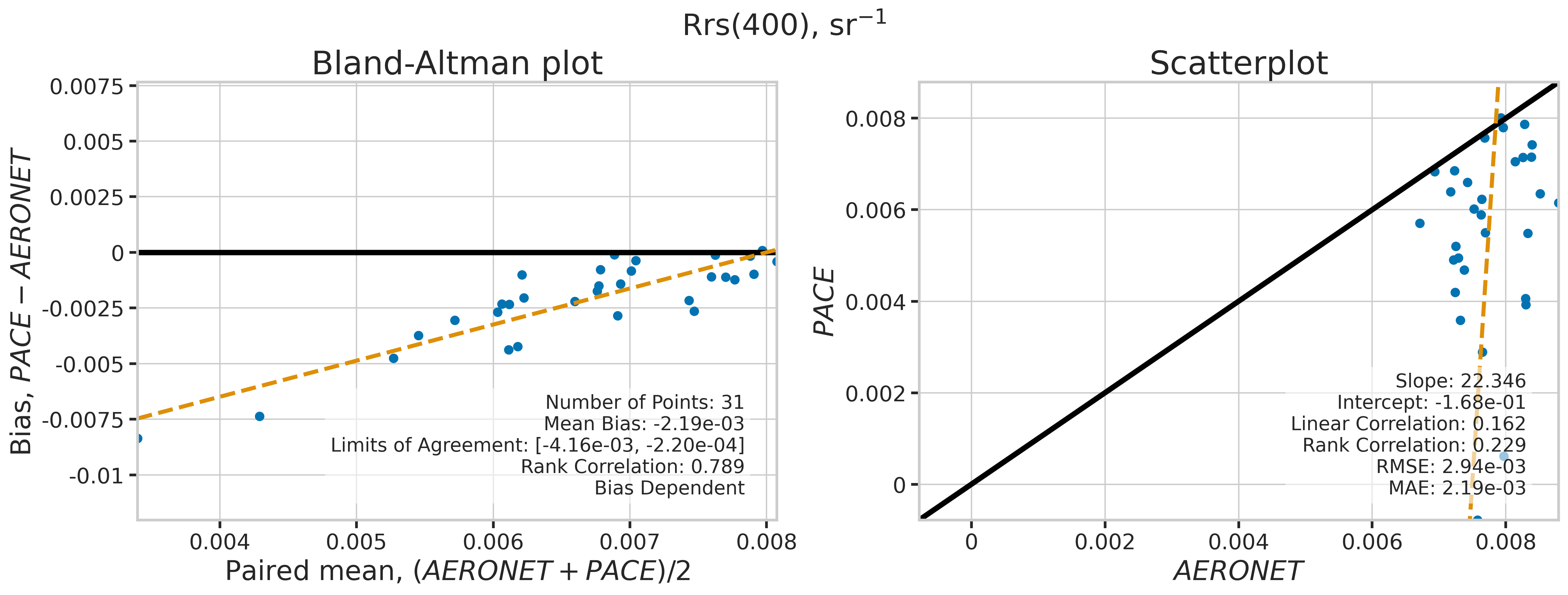
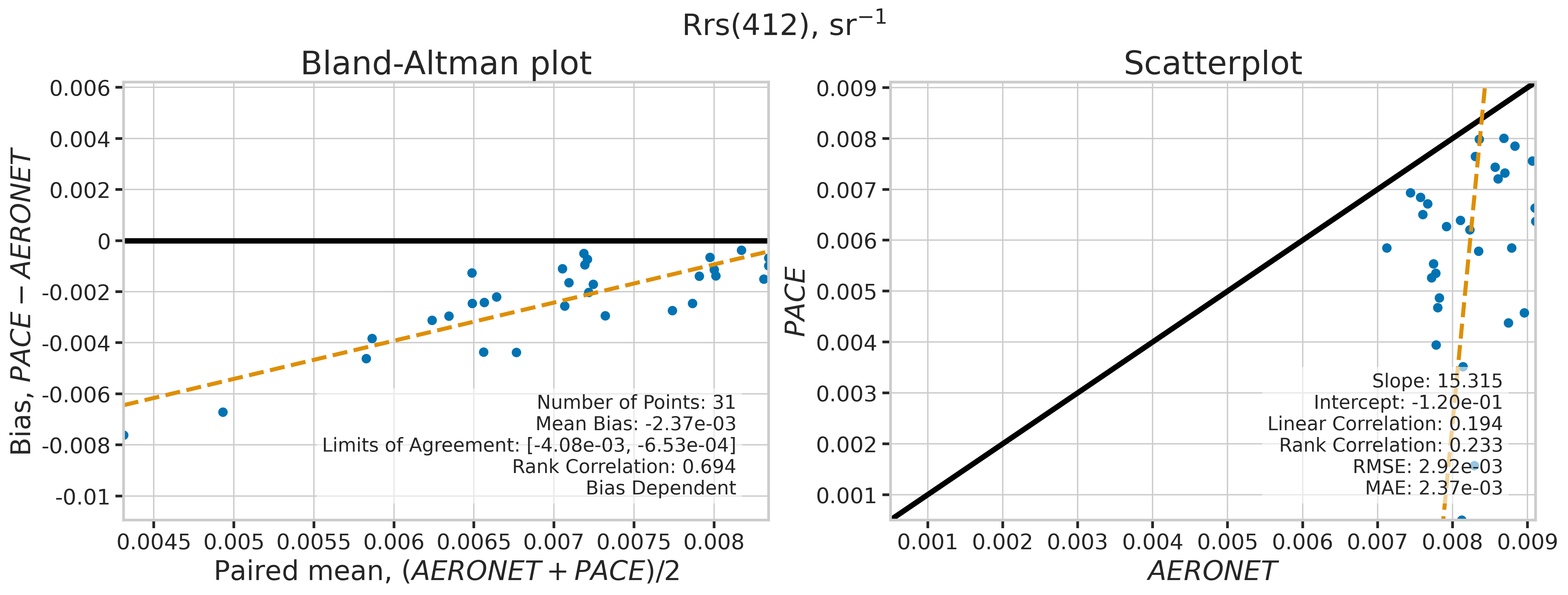
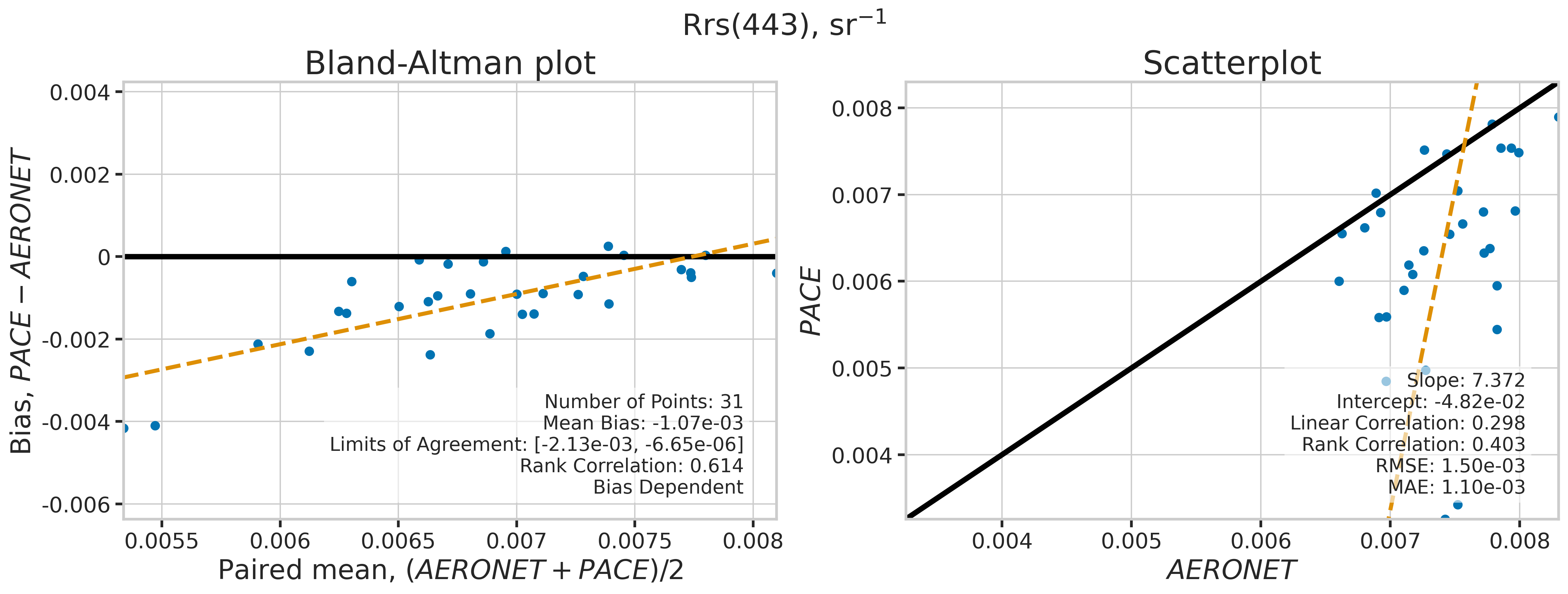
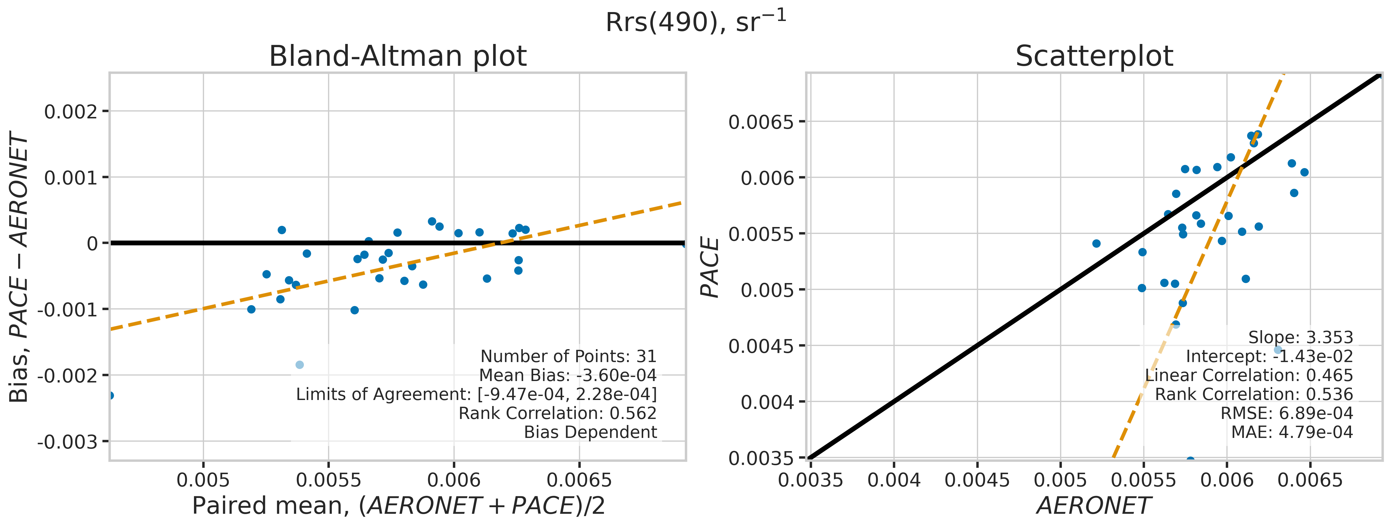
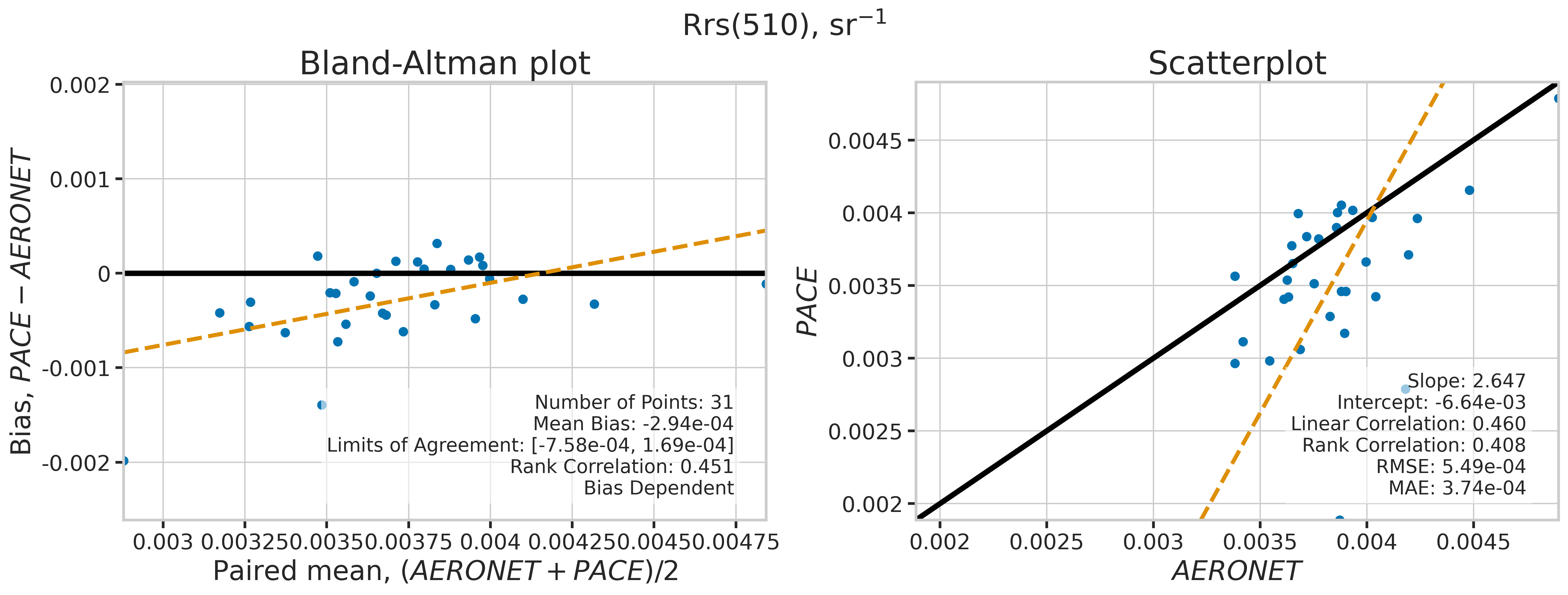
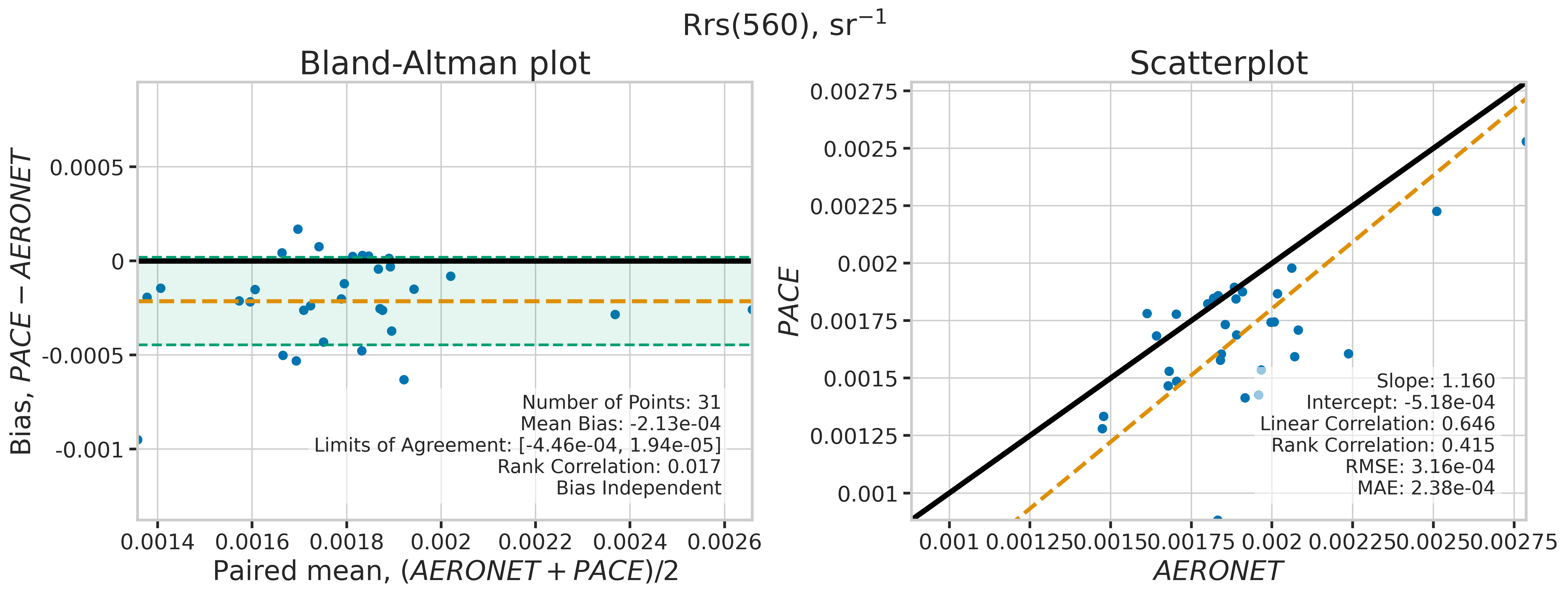
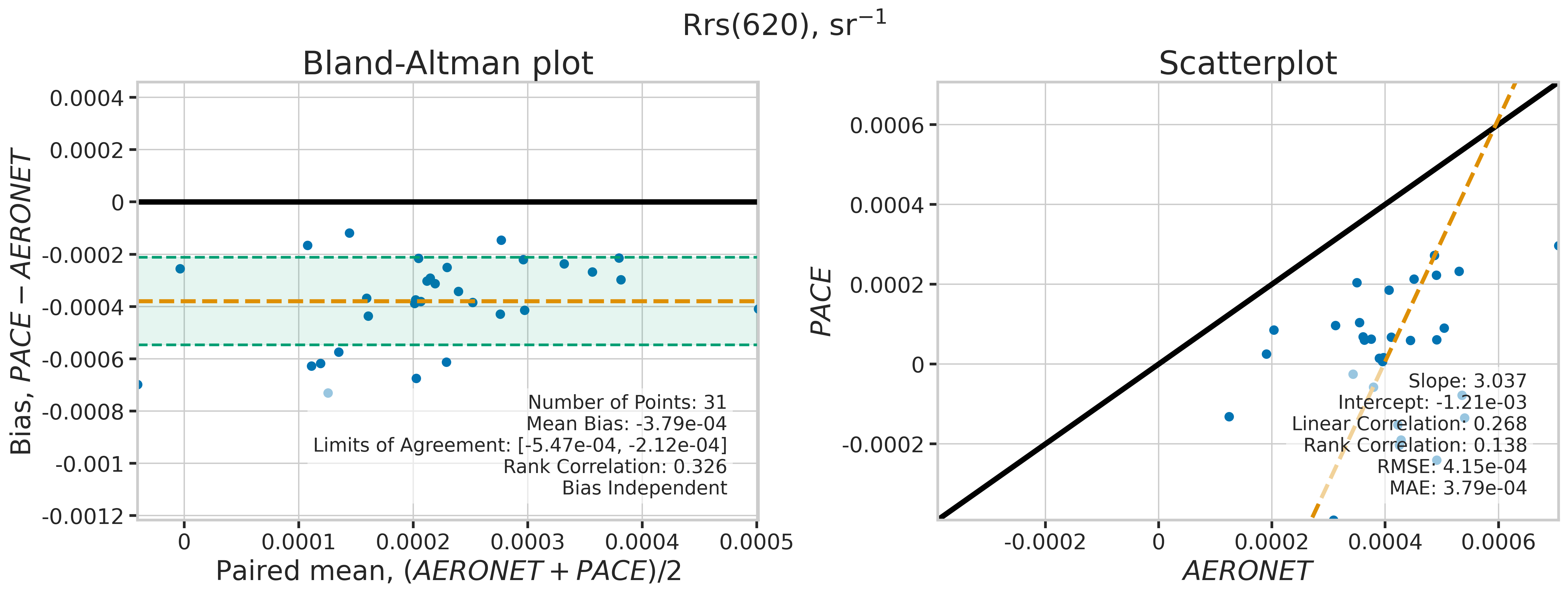
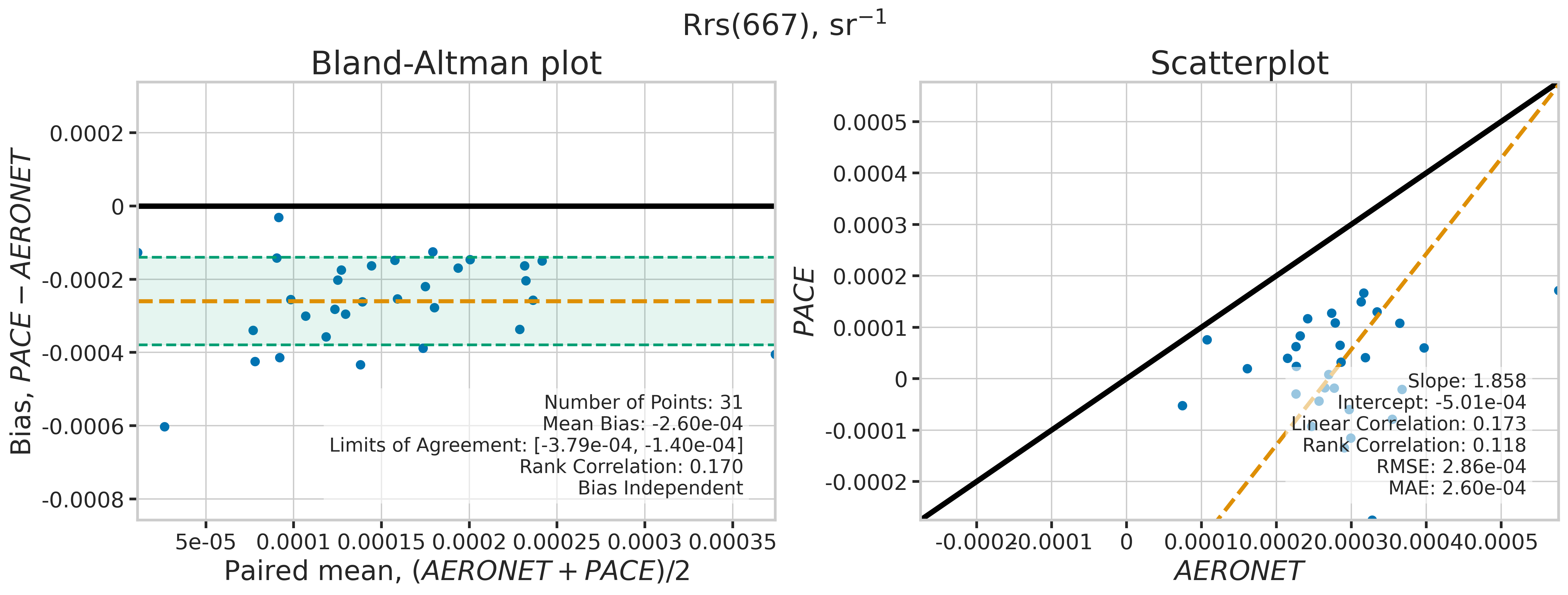
4. Make plots#
We will use the function plot_BAvsScat to plot the paired matchup data as Bland_Altman and scatter plots. The Bland-Altman plots provide insights into the bias and precision of the satellite measurements compared to field measurements. A mean difference close to zero indicates good agreement, while the spread of differences (limits of agreement) puts the bias within the context of the variability of the field data. Additionally, a check is done to assess the scale dependency of the bias, such as errors increasing when the magnitude of the observations increases. If a scale dependency exists, the limits of agreement are replaced with a regression line showing its direction and magnitude. Scatter plots complement Bland-Altman plots by showing the strength of the linear relationship between the two datasets, with high correlation coefficients and low RMSE values indicating strong agreement and high accuracy of the satellite-derived measurements.
?plot_BAvsScat
MATCH_WAVES = np.array([400, 412, 443, 490, 510, 560, 620, 667])

# Loop through matchup wavelengths
stats_list = []
for idx, match_wave in enumerate(MATCH_WAVES):
    # Find matching OCI columns
    idx_sat = np.where(np.abs(waves_sat - match_wave) <= 5)[0]
    match_sat = np.nanmean(rrs_sat[:, idx_sat], axis=1)

    # Find matching AOC columns
    idx_aoc = np.where(np.abs(waves_aoc - match_wave) <= 5)[0]
    match_aoc = np.nanmean(rrs_aoc[:, idx_aoc], axis=1)

    valid_indices = np.isfinite(match_sat) & np.isfinite(match_aoc)
    if np.sum(valid_indices) > 5:
        fig_label = f"Rrs({match_wave}), sr" + r"$\mathregular{^{-1}}$"
        dict_stats = plot_BAvsScat(match_aoc[valid_indices],
                                   match_sat[valid_indices],
                                   label=fig_label,
                                   saveplot=None,
                                   x_label="AERONET", y_label="PACE",
                                   is_type2=True)
        dict_stats["wavelength"] = match_wave
        stats_list.append(dict_stats)

# Organize stats DataFrame
df_stats = pd.DataFrame(stats_list)
df_stats.set_index('wavelength', inplace=True)
df_stats = df_stats.fillna(-999)
df_stats
| Number_of_Points | Scale_Independence | Mean_Bias | Limits_of_Agreement_low | Limits_of_Agreement_high | Linear_Slope | Linear_Intercept | Linear_Correlation | Rank_Correlation | RMSE | MAE | |
|---|---|---|---|---|---|---|---|---|---|---|---|
| wavelength | |||||||||||
| 400 | 31 | False | -0.002188 | -999.000000 | -999.000000 | 22.346014 | -0.167513 | 0.162067 | 0.229032 | 0.002943 | 0.002193 |
| 412 | 31 | False | -0.002368 | -999.000000 | -999.000000 | 15.315123 | -0.120106 | 0.193836 | 0.233065 | 0.002924 | 0.002368 |
| 443 | 31 | False | -0.001067 | -999.000000 | -999.000000 | 7.372392 | -0.048241 | 0.298131 | 0.403226 | 0.001505 | 0.001096 |
| 490 | 31 | False | -0.000360 | -999.000000 | -999.000000 | 3.352709 | -0.014327 | 0.465080 | 0.535887 | 0.000689 | 0.000479 |
| 510 | 31 | False | -0.000294 | -999.000000 | -999.000000 | 2.647192 | -0.006642 | 0.459783 | 0.408065 | 0.000549 | 0.000374 |
| 560 | 31 | True | -0.000213 | -0.000446 | 0.000019 | 1.160110 | -0.000518 | 0.645870 | 0.414919 | 0.000316 | 0.000238 |
| 620 | 31 | True | -0.000379 | -0.000547 | -0.000212 | 3.036933 | -0.001208 | 0.268457 | 0.138306 | 0.000415 | 0.000379 |
| 667 | 31 | True | -0.000260 | -0.000379 | -0.000140 | 1.857914 | -0.000501 | 0.172730 | 0.118145 | 0.000286 | 0.000260 |